How to jointly tune learning rate and weight decay for AdamW

14 minute read

Published: February 19, 2024

TL;DR: AdamW is often considered a method that decouples weight decay and learning rate. In this blog post, we show that this is not true for the specific way AdamW is implemented in Pytorch. We also show how to adapt the tuning strategy in order to fix this: when doubling the learning rate, the weight decay should be halved.

Introduction

Consider the training problem

\[\nonumber \min_{w\in \mathbb{R}^d} \ell(w),\]

where $\ell: \mathbb{R}^d\to \mathbb{R}$ is a loss function, and $w$ are learnable parameters. Assume that the loss is given as $\ell(w) = \mathbb{E}_{x\sim \mathcal{P}} [\ell(w,x)]$, where $x$ is a batch of data, sampled from the training data distribution $\mathcal{P}$.

Suppose we want to solve this problem with stochastic gradient methods. Let us introduce some notation: we denote

the initial learning rate by $\alpha > 0$,
the multiplicative learning rate scheduler by $\eta_t > 0$ with $\eta_0=1$,
the weight decay parameter by $\lambda \geq 0$.

The learning rate in iteration $t$ will be given by $\alpha_t := \alpha \eta_t$. We will often refer to $\alpha$ as learning rate parameter, which is slightly inprecise, but for most of the contents the schedule $\eta_t$ will be constant anyway.

The arguably most widely used method for training large-scale machine learning models is AdamW. It has been proposed by Loshchilov and Hutter and its main feature is that it handles weight decay separate from the loss $\ell$ (as opposed to the original Adam [3]). For readers not familiar with AdamW, we refer to [1] and briefly explain the AdamW update formula below.

A short outline of this post:

We explain the AdamW algorithm, and show that it is implemented in Pytorch slightly differently from the original paper.
We explain the notion of decoupling of weight decay and learning rate, and why it is important in practice.
We show why AdamW in Pytorch does not actually decouple weight decay and learning rate, because of the implementation difference mentioned in the first bullet.
We then show how the tuning strategy needs to be adapted in order to fix this.

Disclaimer: I have previously written a blog post for the ICLR 2023 blog post track [2], that discusses the weight decay mechanism of AdamW, and how it can be seen as a proximal version of Adam (the blog post is based on the paper by Zhuang et al [4]). This post will re-use some of the figures and contents. In fact, I stumbled upon the central question of this blog post during writing back then.

On the subtleties of implementing `AdamW`

The quantities involed in AdamW are mostly the same as in the original version of Adam: let $g_t=\nabla \ell(w_t,x_t)$ be the stochastic gradient in iteration $t$, then for $\beta_1,\beta_2\in[0,1)$ we compute

\[m_t = \beta_1 m_{t-1} + (1-\beta_1) g_t, \nonumber \\ v_t = \beta_2 v_{t-1} + (1-\beta_2) g_t \odot g_t. \nonumber \\\]

The bias-corrected quantities are then given by

\[\hat m_t = m_{t}/(1-\beta_1^{t}), \nonumber \\ \hat v_t = v_{t}/(1-\beta_2^{t}) . \nonumber \\\]

Let us denote the Adam preconditioner by $D_t = \mathrm{diag}(\epsilon + \sqrt{\hat v_t})$. The way that AdamW was proposed originally in the paper by Loshchilov and Hutter [1] is

\[w_{t+1} = (1-\lambda\eta_t)w_t - \alpha_t D_t^{-1}\hat m_t. \tag{AdamW-LH}\]

In Pytorch, the method is implemented slightly differently:

\[w_{t+1} = (1-\lambda\alpha_t)w_t - \alpha_t D_t^{-1}\hat m_t. \tag{AdamW-PT}\]

Note that the only difference consists in the coefficient $1-\lambda\alpha_t= 1-\lambda\alpha\eta_t$ instead of $1-\lambda\eta_t$. While this seems like trivia at first sight (one could easily reparametrize $\lambda$ by $\lambda \alpha)$, we will show that it has an important practical implication on tuning.

Remark: The implementation of AdamW is the same in Optax as in Pytorch. Hence, what follows applies similarly to tuning AdamW in Optax.

The meaning of decoupling

So what do we mean when we say that learning rate $\alpha$ and weight decay $\lambda$ are decoupled? We will work with the following (approximate) definition: we say that $\alpha$ and $\lambda$ are decoupled, if the optimal choice for $\lambda$ does not depend on the choice of $\alpha$. Here, we mean optimal with respect to some metric of interest - for the rest of the blog post, this metric will be the loss $\ell$ computed over a validation dataset.

The graphic below illustrates this phenomenon: imagine, we draw a heatmap of the validation loss over a $(\alpha,\lambda)$ grid. Bright values indicate a better model performance. Then, in a coupled scenario (left) the bright valley could have a diagonal shape, while for the decoupled scenario (right) the valley is more rectangular.

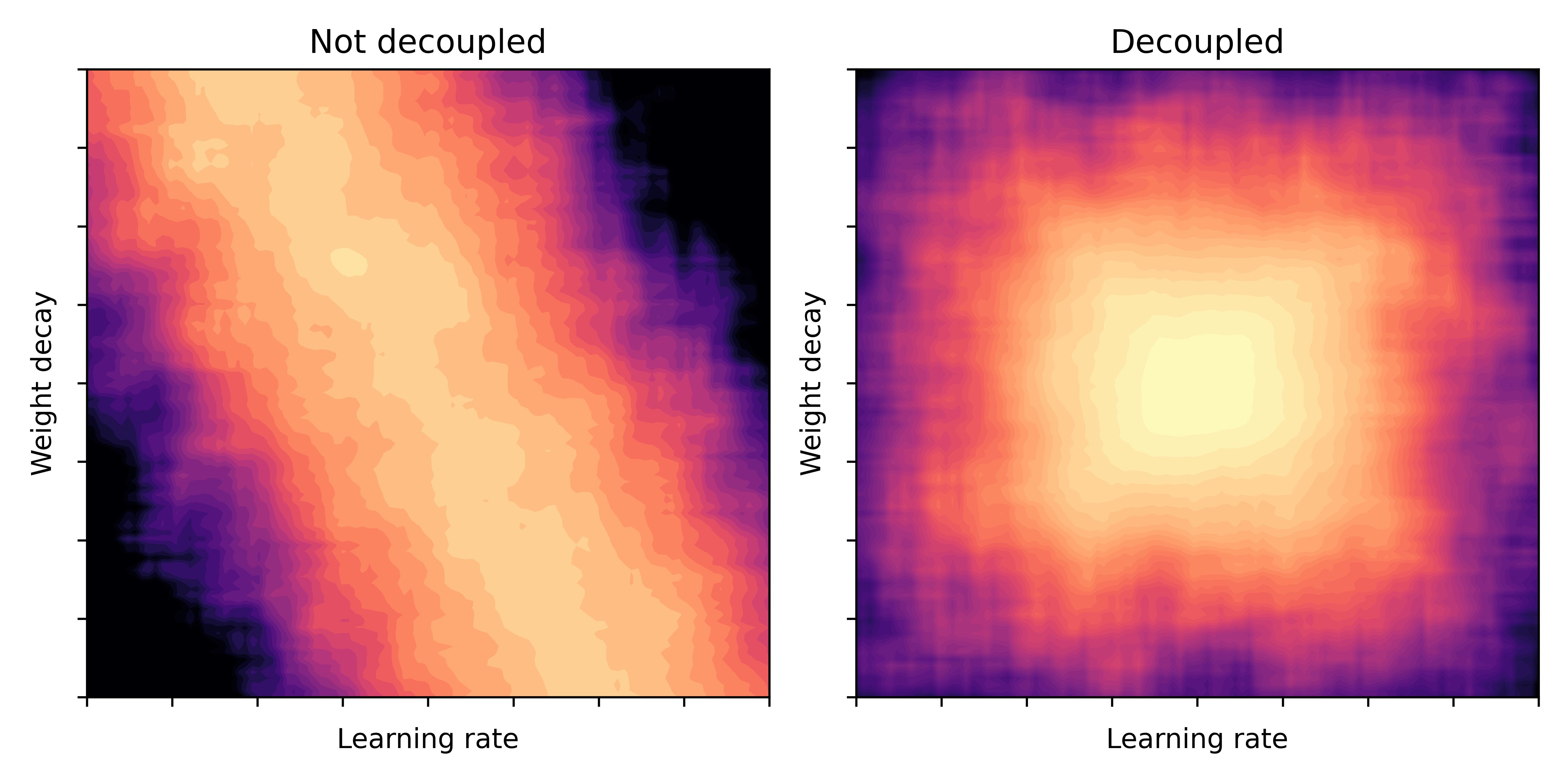Fig. 1: Model performance (bright = good) as a function of learning rate and weight decay parameters. Illustration taken from [2].

Note that in practice this can make a huge difference: in general, we need to tune over the 2D-space of $(\alpha,\lambda)$, assuming that all other hyperparameters are already set. The naive way to do this is a grid search. However, if we know that $\alpha$ and $\lambda$ are decoupled, then it would be sufficient to do two separate line searches for $\alpha$ and $\lambda$, followed by combining the best values from each line search. For example, if for each parameter we have $N$ candidate values, this reduces the tuning effort from $N^2$ (naive grid search) to $2N$ (two line searches).

This motivates why the decoupling property is important for practical use.

AdamW and its promise of decoupling

One of the main contributions of the AdamW paper [1] was that it showed how to treat weight decay separately from the loss. This is declared in the paper as follows:

The main contribution of this paper is to improve regularization in Adam by decoupling the weight decay from the gradient-based update.

The authors also claim that their method decouples the weight decay parameter $\lambda$ and the learning rate $\alpha$ (which goes beyond decoupling weight decay and loss).

We provide empirical evidence that our proposed modification decouples the optimal choice of weight decay factor from the setting of the learning rate for […] Adam.

While this claim is supported by experiments in the paper, we will show next an example where there is no decoupling when using AdamW from Pytorch. The reason for this is, as we will show, the implementation subtlety we described in the previous section.

A simple experiment

The experiment is as follows: we solve a ridge regression problem for some synthetic data $A \in \mathbb{R}^{n \times d},~b\in \mathbb{R}^{n}$ with $n=200,~d=1000$. Hence $\ell$ is the squared loss, given by $\ell(w) = \Vert Aw-b \Vert^2$.

We run both AdamW-LH and AdamW-PT, for a grid of learning-rate values $\alpha$ and weight-decay values $\lambda$. For now, we set the scheduler to be constant, that is $\eta_t=1$. We run everything for 50 epochs, with batch size 20, and average all results over five seeds.

Below is the final validation-set loss, plotted as heatmap over $\alpha$ and $\lambda$. Again, brighter values indicate lower loss values.

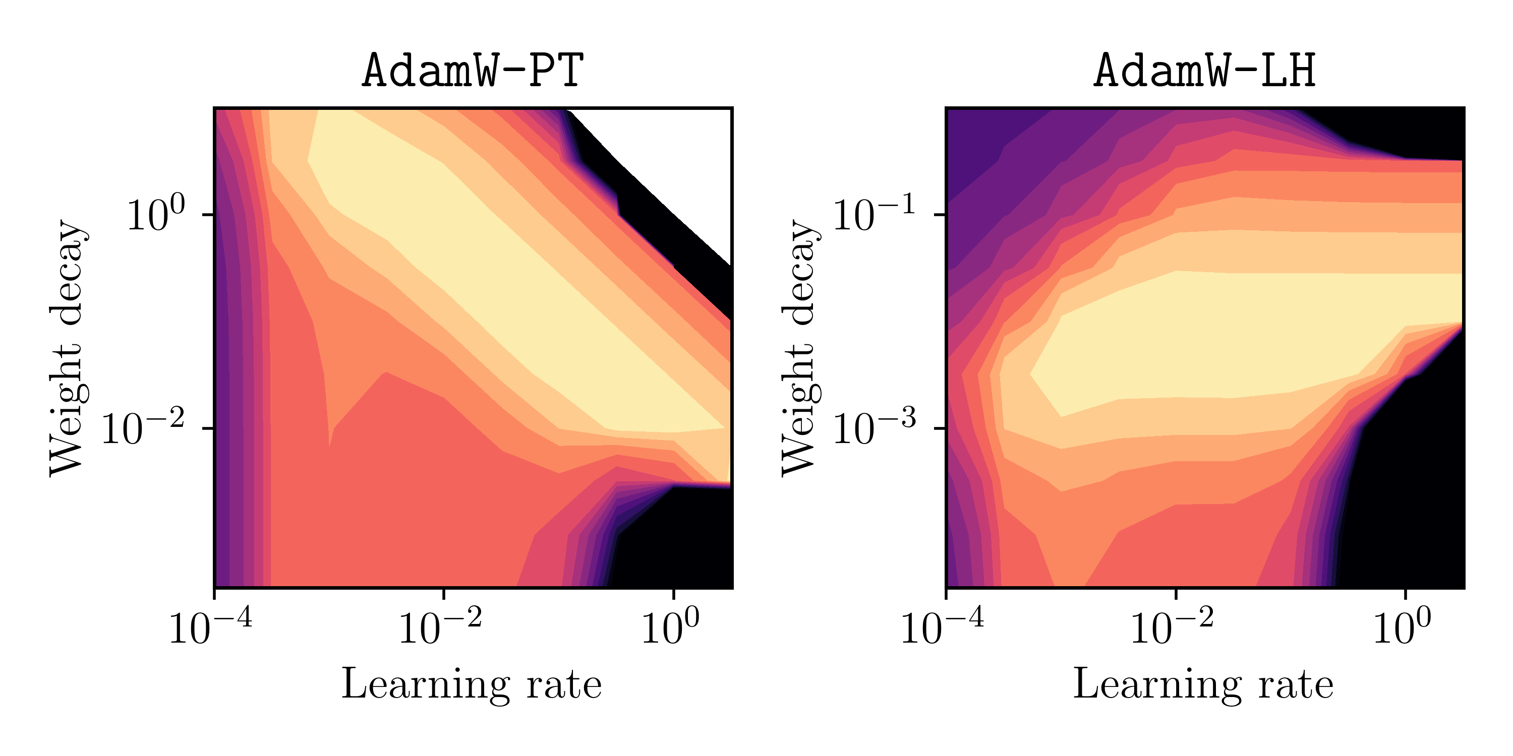Fig. 2: Final validation loss (bright = low) as a function of learning rate $\alpha$ and weight decay parameter $\lambda$.

This matches the previous illustrative picture in Figure 1 pretty well (it’s not a perfect rectangle for AdamW-LH, but I guess it proves the point)!

Conclusion 1: Using the Pytorch implementation AdamW-PT, the parameters choices for $\alpha$ and $\lambda$ are not decoupled in general. However, the originally proposed method AdamW-LH indeed shows decoupling for the above example.

Based on this insight, the obvious question is: what is the best (joint) tuning strategy when using the Pytorch version AdamW-PT? We answer this next.

The right tuning strategy

Assume that we have already found a good candidate value $\bar \lambda$ for the weight-decay parameter; for example, we obtained $\bar \lambda$ by tuning for a fixed (initial) learning rate $\bar \alpha$. Now we also want to tune the (initial) learning-rate value $\alpha$.

Assume that our tuning budget only allows for one line search/sweep. We will present two options for tuning:

(S1) Keep $\lambda = \bar \lambda$ fixed, and simply sweep over a range of values for $\alpha$.

If $\alpha$ and $\lambda$ are decoupled, then (S1) should work fine. However, as we saw before, the Pytorch version of AdamW, called AdamW-PT, seems not to be decoupled. Instead, the decay coefficient in each iteration is given by $1 - \alpha \lambda \eta_t$. Thus, it seems intuitive to keep the quantity $\alpha \lambda$ fixed, which is implemented by the following strategy:

(S2) When sweeping over $\alpha$, adapt $\lambda$ accordingly such that the product $\alpha \lambda$ stays fixed. For example, if $\alpha = 2\bar \alpha$, then set $\lambda=\frac12 \bar \lambda$.

Strategy (S1) is slightly easier to code; my conjecture is that (S1) is also employed more often than (S2) in practice.

However, and this is the main argument, from the way AdamW-PT is implemented, (S2) seems to be more reasonable. We verify this next.

We plot again the heatmaps as before, but now highlighting the points that we would actually observe by the tuning strategy (S1) or (S2). We show below

left: (S1) for AdamW-PT ,
middle: (S2) for AdamW-PT,
right: (S1) for AdamW-LH (as we had seen that AdamW-LH is indeed decoupled).

Here, we set $(\bar \lambda, \bar \alpha) =$ (1e-2,3.2e-1) for AdamW-PT, and $(\bar \lambda, \bar \alpha) =$ (1e-2,3.2e-3) for AdamW-LH. In the below plots, the circle-shaped markers highlight the sweep that corresponds to the tuning strategy (S1) or (S2). The bottom plot shows the validation loss as a curve over the highlighted markers.

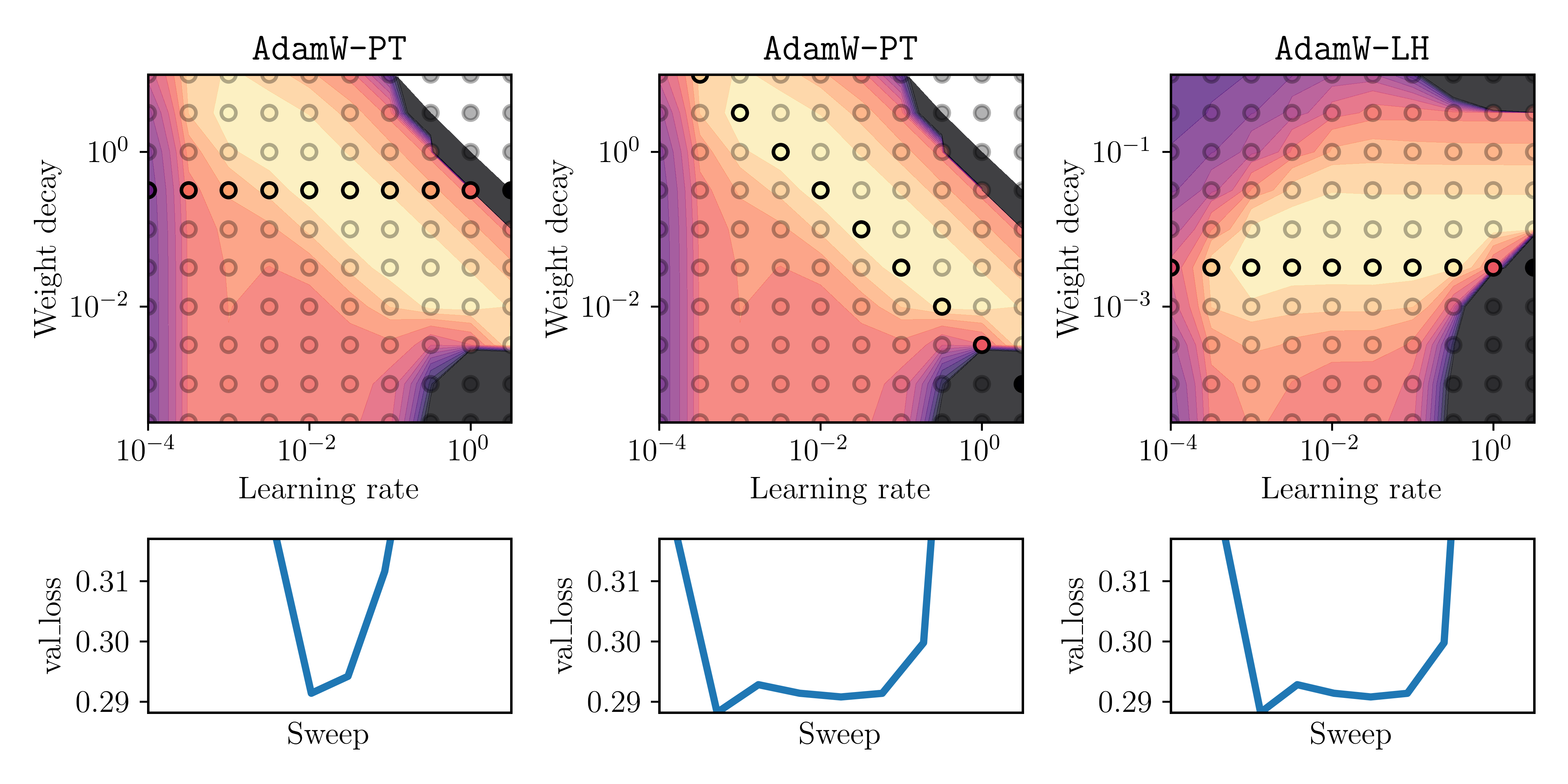Fig. 3: Three different tuning strategies: (S1) for AdamW-PT (left), (S2) for AdamW-PT (middle) and (S1) for AdamW-LH (right). Top: Heatmap of final validation loss where the highlighted points show the results of the respective sweep. Bottom: A curve of the final validation loss at each of the highlighted points (learning rate increases from left to right on x-axis).

Note that the bottom plot displays the final validation-loss values that a practitioner would observe for the sweep of each respective tuning strategy. What is important is the width of the valley of this curve, as it reflects how dense the sweep would need to be to obtain a low final loss. The main insight here is: for the middle and right ones, it would be much easier to obtain a low final loss, as for the left one. This is important when the sweep has only few trials due to high computational costs for a single run, or other practical constraints.

Conclusion 2: when using the Pytorch version of AdamW (i.e. AdamW-PT), tuning strategy (S2) should be used. That is, when doubling the learning rate, the weight decay should be halved.

In fact, Figure 3 also shows that tuning strategy (S2) for AdamW-PT is essentially the same as strategy (S1) for AdamW-LH.

Summary and final remarks:

Implementation details can have an effect on hyperparameter tuning strategies. We showed this phenomenon for AdamW, where the tuning strategy should be a diagonal line search if the Pytorch implementation is used.
In the appendix, we show that the results are similar when using a square-root decaying scheduler for $\eta_t$ instead.
This blog post only covers a ridge regression problem, and one might argue that the results could be different for other tasks. However, the exercise certainly shows there is no decoupling for AdamW-PT for one of the simplest possible problems, ridge regression. I also observed good performance of the (S2) strategy for AdamW-PT when training a vision transfomer on Imagenet (with the timm library).

If you want to cite this post, please use

@misc{adamw-decoupling-blog,
      title = {How to jointly tune learning rate and weight decay for {A}dam{W}},
      author = {Schaipp, Fabian},
      howpublished = {\url{https://fabian-sp.github.io/posts/2024/02/decoupling/}},
      year = {2024}
    }

References

[1] Loshchilov, I. and Hutter, F., Decoupled Weight Decay Regularization, ICLR 2019.

[2] Schaipp F., Decay No More, ICLR Blog Post Track 2023.

[3] Kingma, D. and Ba, J., Adam: A Method for Stochastic Optimization, ICLR 2015.

[4] Zhuang Z., Liu M., Cutkosky A., Orabona F., Understanding AdamW through Proximal Methods and Scale-Freeness, TMLR 2022.

Appendix

Results with square-root schedule

To validate that the effects are similar for non-constant learning rates, we run the same experiment but now with a square-root decaying learning rate schedule. That is $\eta_t = 1/\sqrt{\text{epoch of iteration } t}$. We sweep again over the initial learning rate $\alpha$ and weight decay parameter $\lambda$. The results are plotted below:

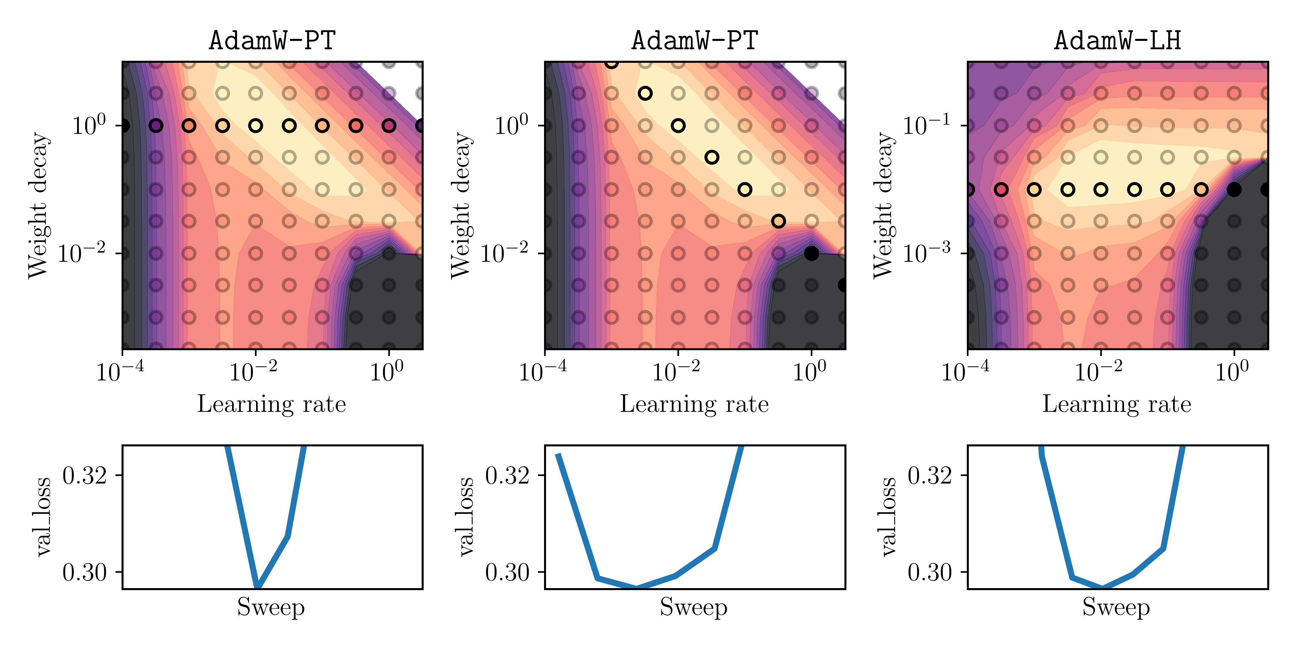Fig. 4: Same as Figure 3, but with a square-root decaying learning-rate schedule.

Pytorch code for `AdamW-LH`

For completeness, this is the code we used for AdamW-LH. It is adapted from here.

class AdamLH(Optimizer):
    """ AdamW with fully decoupled weight decay.
    """

    def __init__(self, params, lr=1e-3, betas=(0.9, 0.999), eps=1e-8,
                 weight_decay=0):
        if not 0.0 <= lr:
            raise ValueError("Invalid learning rate: {}".format(lr))
        if not 0.0 <= eps:
            raise ValueError("Invalid epsilon value: {}".format(eps))
        if not 0.0 <= betas[0] < 1.0:
            raise ValueError("Invalid beta parameter at index 0: {}".format(betas[0]))
        if not 0.0 <= betas[1] < 1.0:
            raise ValueError("Invalid beta parameter at index 1: {}".format(betas[1]))
        if not 0.0 <= weight_decay:
            raise ValueError("Invalid weight_decay value: {}".format(weight_decay))
        
        defaults = dict(lr=lr, betas=betas, eps=eps, weight_decay=weight_decay)
        
        self._init_lr = lr
        super(AdamLH, self).__init__(params, defaults)

    def __setstate__(self, state):
        super(AdamLH, self).__setstate__(state)
        for group in self.param_groups:
            group.setdefault('amsgrad', False)

    @torch.no_grad()
    def step(self, closure=None):
        """
        Performs a single optimization step.

        Parameters
        ----------
        closure : LossClosure, optional
            A callable that evaluates the model (possibly with backprop) and returns the loss,
            by default None.
        
        loss : torch.tensor, optional
            The loss tensor. Use this when the backward step has already been performed.
            By default None.
        

        Returns
        -------
        (Stochastic) Loss function value.
        """
        loss = None
        if closure is not None:
            with torch.enable_grad():
                loss = closure()

        for group in self.param_groups:
            lr = group['lr']
            lmbda = group['weight_decay']
            eps = group['eps']
            beta1, beta2 = group['betas']

            for p in group['params']:
                if p.grad is None:
                    continue
                
                # decay
                p.mul_(1 - lmbda*lr/self._init_lr)

                grad = p.grad
                
                state = self.state[p]

                # State initialization
                if len(state) == 0:
                    state['step'] = 0
                    # Exponential moving average of gradient values
                    state['exp_avg'] = torch.zeros_like(p, memory_format=torch.preserve_format)
                    # Exponential moving average of squared gradient values
                    state['exp_avg_sq'] = torch.zeros_like(p, memory_format=torch.preserve_format)
                    
                exp_avg, exp_avg_sq = state['exp_avg'], state['exp_avg_sq']
                
                state['step'] += 1
                bias_correction1 = 1 - beta1 ** state['step']
                bias_correction2 = 1 - beta2 ** state['step']


                # Decay the first and second moment running average coefficient
                exp_avg.mul_(beta1).add_(grad, alpha=1-beta1)
                exp_avg_sq.mul_(beta2).addcmul_(grad, grad, value=1-beta2)
                
                denom = (exp_avg_sq.sqrt() / math.sqrt(bias_correction2)).add_(eps)

                step_size = lr / bias_correction1
                update = -step_size * exp_avg / denom
                p.add_(update)
                
        return loss

Share on

Twitter Facebook LinkedIn

Fabian Schaipp

How to jointly tune learning rate and weight decay for AdamW

Introduction

On the subtleties of implementing `AdamW`