
Infinite Schedules and the Benefits of Lookahead
Published:
TL;DR: Knowing the next training checkpoint in advance (“lookahead”) helps to set the learning rate. In the limit, the classical square-root schedule appears on the horizon.
Introduction
In this ICML 2025 paper, we showed that the behaviour of learning-rate schedules in deep learning can be explained - perhaps surprisingly - with convex optimization theory. This can be exploited to design better schedules: for example, we show that a schedule which we designed based on the theory (hence, for free) gives significant improvements for continual LLM training (~7% of steps saved for 124M and 210M Llama-type models, see Section 5.1 in the paper for details).
In the paper, we specifically designed a schedule for a two-stage continual learning scenario. Our proposed schedule is piecewise constant in each stage (combined with warmup and linear cooldown in the end).
In this blog post, we ask ourselves the question: what happens with more than two stages? What is the limiting behaviour?
Disclaimer: in contrast to the paper, where we tested these schedules on actual LLM pretraining tasks, here we will only look at their theoretical performance in terms of a worst-case suboptimality bound (see Figure 2 for the concrete bound).
Setup (Part I)
Let us consider the iterates of SGD given by
\[x_{t+1} = x_t - \gamma \eta_t g_t,\]where \( (\eta_t)_{t\in \mathbb{N}}\) is a sequence of positive reals, \(\gamma > 0 \) and \(g_t\) is the (batch) gradient of our loss function.
Note that we decompose the step size into a base learning-rate \(\gamma\) and a schedule \((\eta_t)_t\). In a Pytorch training script, these two objects resemble lr (passed to the optimizer) and the torch.optim.lr_scheduler.
Recap
We give a quick summary of our experiment in the paper, which will be the starting point of this blog post. For more background, see Section 5.1 of the paper.
Consider the following scenario: we have previously trained a model for \(T_1\) steps. Now, we want to continue training up to \(T_2>T_1\) steps, but reuse the checkpoint after \(T_1\) steps instead of starting from scratch.
The problem: with increasing training horizon, the optimal base learning-rate \(\gamma\) decreases. This is true in theory and practice. So, if we had tuned our base learning-rate \(\gamma\) for the short run (which we assume here), it will be suboptimal for the long run.
Our solution is to adapt the schedule \((\eta_t)_t\) between \(T_1\) and \(T_2\), so that we can keep the base learning rate the same. Specifically, we construct a piecewise constant schedule which decreases in the second stage of training (from \(T_1\) to \(T_2\)). The decreasing factor is computed such that the optimal base LR \(\gamma\) (tuned in the first stage) remains the same, according to the bound from convex optimization theory. This computation can be done effectively for free.
This piecewise constant schedule is combined with a WSD-like approach (warmup-stable-decay), which uses a short warmup and linear cooldown to zero over the final 20% of steps. In our experiments we set \(T_1=50k\) and tried both \(T_2\in \{100k,200k\}\). Figure 1 below shows that this adapted schedule leads to an improvement in LLM pretraining, compared to keeping the schedule unmodified for the longer horizon.1
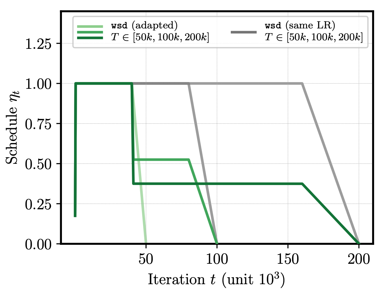
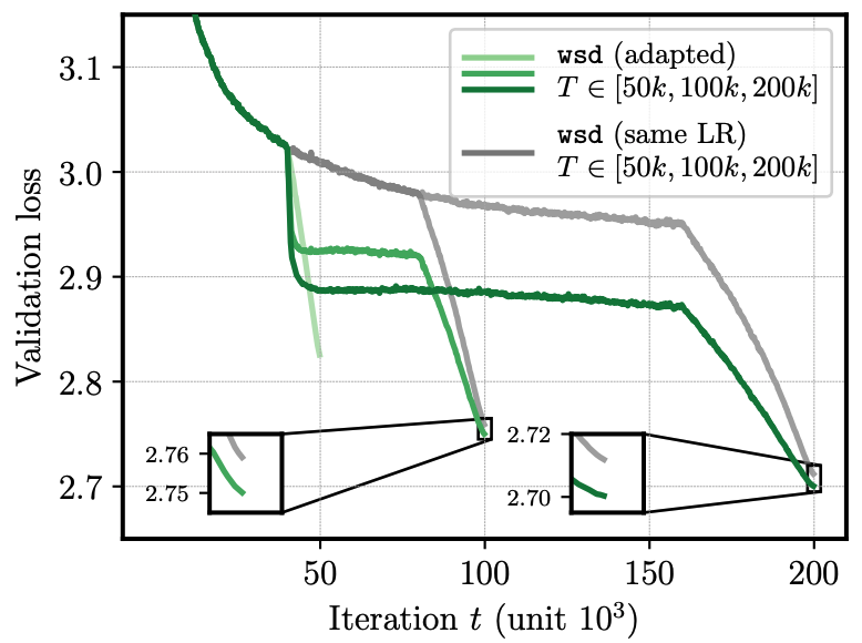
Figure 1 (from Schaipp et al., 2025): When extending the training horizon T from 50k to 100k or 200k steps, the piecewise constant schedule (left, green) constructed from theory achieves loss improvement for LLM pretraining compared to baseline (grey).
This brings us to the main question of this blog post: what happens if we go beyond two stages of training? What is the limiting schedule if we do the same sequentially for training horizons \(T_1 < T_2<\cdots<T_n\) and \(n\to +\infty\)?
Setup (Part II)
Let \(n\in \mathbb{N}\) and \(\Delta t\in \mathbb{N}\). The starting point is indexed with \(t=1\).2 Assume that we train in total for \(n\) stages, defined by the checkpoints \(T_k = 1+ k \cdot \Delta t\) with \(k=1,\ldots,n\).
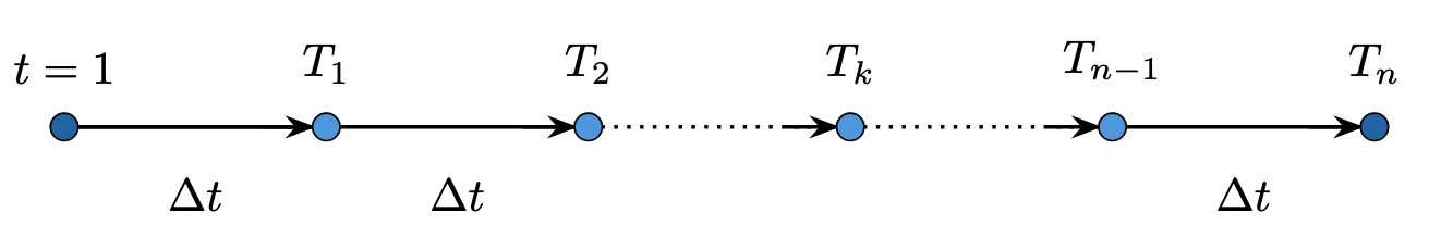
We focus on three different schedules (depicted in the animation further above):
1) Piecewise constant. This schedule is constructed sequentially: at each checkpoint \(T_k\), we decide on the next stage up to \(T_{k+1}\). During each stage, the schedule is constant (but at decreasing values). As described above and in the paper, we compute the decreasing factor stage-by-stage based on the theory, in order to keep the optimal base LR as close to theoretically optimal as possible.
2) Sqrt. Schedule set as \(\eta_t = 1/\sqrt{t}\). In the convex, Lipschitz-continuous setting, it achieves a last-iterate bound of \(\frac{DG}{2\sqrt{T}} \mathcal{O}(\log(T)^{1/2})\) (Orabona 2020, see further details below in the Appendix).
3) Linear-decay. For each \(k=1,\ldots,n\), we construct a schedule that decreases linearly from 1 to 0 over the interval \([1, T_k]\). Thus, for each checkpoint/horizon \(T_k\), the resulting schedule is different, which in practice would require retraining from scratch.
Notice that for linear-decay we construct a different schedule for each checkpoint/training horizon \(T_k\) (\(k=1,\ldots,n\)); in contrast to this, we construct only one single piecewise constant and sqrt schedule that covers \([1,T_n]\). One could call these “anytime schedules”, or “infinite schedules” (Zhai et al., 2022) as \(T_n\) can be arbitrarily large.
The notion of look-ahead. We should also point out that these three schedules are different in the way that they have knowledge of the training horizon: the sqrt is fully independent of the horizon; linear-decay is fully dependent on the horizon; the piecewise constant schedule lies in between, as it is constructed sequentially and only needs to know the next checkpoint in advance.
In other words, the three schedule differ in how far they can look-ahead the training horizon. On the one extreme, the sqrt schedule can only plan ahead until the next step, on the other extreme the linear-decay schedule can plan ahead for the entire training horizon (see Table 1). Knowledge on the training horizon can lead to better performance (or bounds).
| Schedule | Look-ahead (number of steps) |
|---|---|
| Sqrt | 1 |
| Piecewise constant | \(\Delta t\) |
| Linear-decay | \(T_k\) |
We will evaluate the theoretical bound from our paper (see Theorem 3.1 therein, or Figure 2 below) for each of the three schedule candidates. The central questions are:
(i) how much improvement (in terms of the bound) do we achieve by looking ahead further? This can be indicative for real-world performance (based on the conclusions from our paper).
(ii) What happens in the limit when \(n \to \infty\)? What are the asymptotics of the piecewise constant schedule?
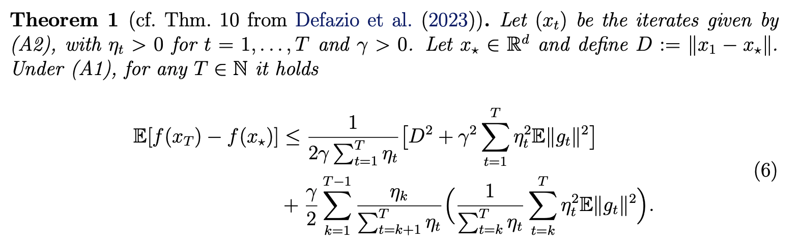
Figure 2 (from Schaipp et al., 2025): Theoretical bound for SGD with arbitrary schedule in convex, nonsmooth optimization.
Tuning the base-learning rate. Before going to results, it remains open how we choose the base learning-rate \(\gamma\) for each of the schedules:
For the piecewise constant schedule, we pick the \(\gamma\) that minimizes the bound at the first checkpoint \(T_1\) when setting \(D=G=1\). (Here, \(G\) denotes an upper bound of the gradient norms \(\|g_t\| \).) We then keep this value of \(\gamma\) for the rest of training until \(T_n\).
For the sqrt-schedule, we do the same as for piecewise constant in order to allow a fair comparison; note that this tuning of \(\gamma\) implicitly introduces some look-ahead for this schedule, however only during the first stage of training up to \(T_1\). In contrast, the piecewise constant schedule has a look-ahead advantage for the entire rest \([T_1, T_n]\) as well.
For linear-decay remember that we construct a schedule for each checkpoint/horizon \(T_k\) with \(k\in[n]\). Accordingly, we pick \(\gamma_k\) for each \(k=1,\ldots,n\) such that it minimizes the bound for the respective \(T_k\) (again setting \(D=G=1\)).
One subtlety here is that the optimal value of \(\gamma\) requires knowledge of \(D\) and \(G\); through the above tuning procedure we allow all three schedule implicit knowledge of these values. (I made sure manually that the specific values of \(D\) and \(G\) do not affect the results below qualitatively.)
Warmup and cooldown. To keep things simple, we did not include neither warmup nor cooldown for the schedules here.
Results
We first set \(\Delta t =100\) and \(n\) such that \(T_n=10\,000\). First, let us compare the piecewise constant schedule to the linear-decay schedule(s).
Performance gap to linear-decay. Figure 3 reveals that the piecewise constant schedule (blue) performs worse than linear-decay (greys) for each single horizon \(T_k\). This is not surprising: linear-decay is known to achieve the best worst-case bound (Defazio et al., 2023; Zamani & Glineur, 2023), and as it can plan for the entire horizon, it should also yield better performance.
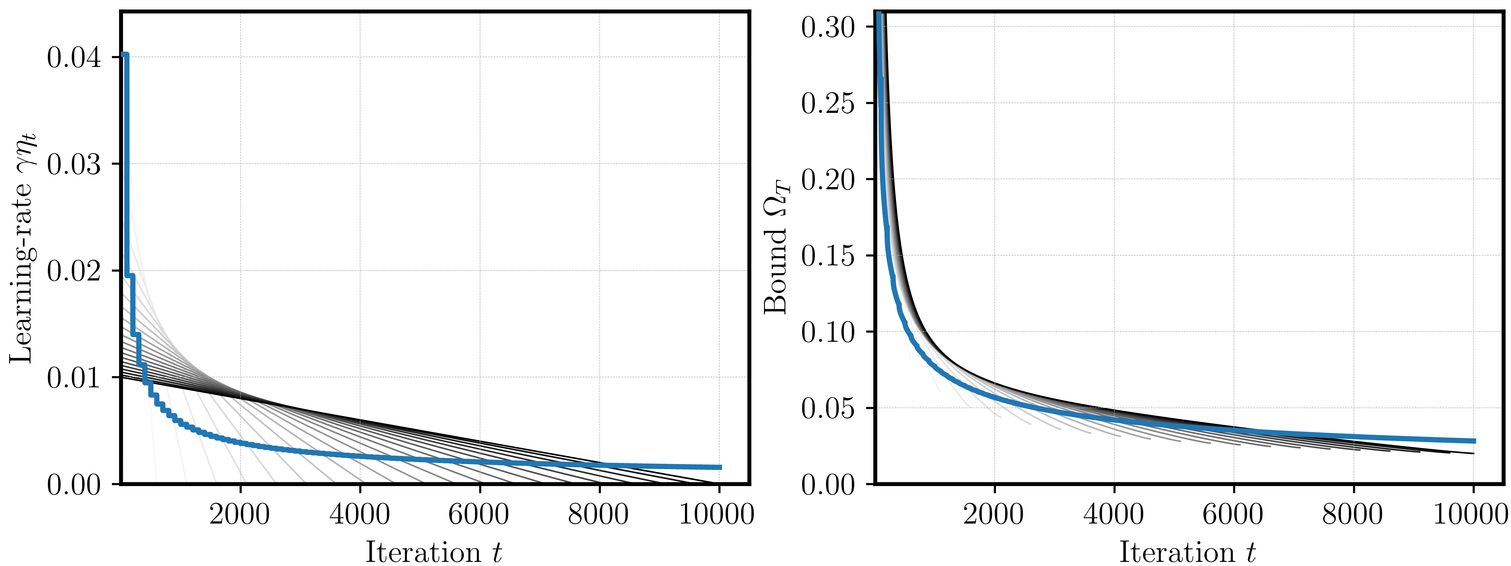
Figure 3: Piecewise constant schedule (blue) performs worse than linear-decay (greys).
So how big is the gap in terms of the convergence rate? Here, it seems appropriate to fit a “scaling law”: let \(y_T\) be the ratio of the final bound \(\Omega_{T}\) for \(k=1,\ldots,n\) of the two schedules. Then, we can fit \(y_T\) as a function of \(T\) based on our observations at \(T_k,~k=1,\ldots,n\). We fit two laws:
\[ y_T = a + b \cdot T^c, \quad y_T = a + b\cdot \log(T)^c \]
Here, \(a,b,c\) are fittable parameters, and we constrain \(a,b\) to be positive; for the second law, we constrain \(c\in [-\infty.1]\). The powerlaw wrt \(\log(T)\) is motivated by the fact that log-factors often appear for slightly suboptimal schedules (for example, a cooldown also brings \(\sqrt{\log(T)}\) of improvement).
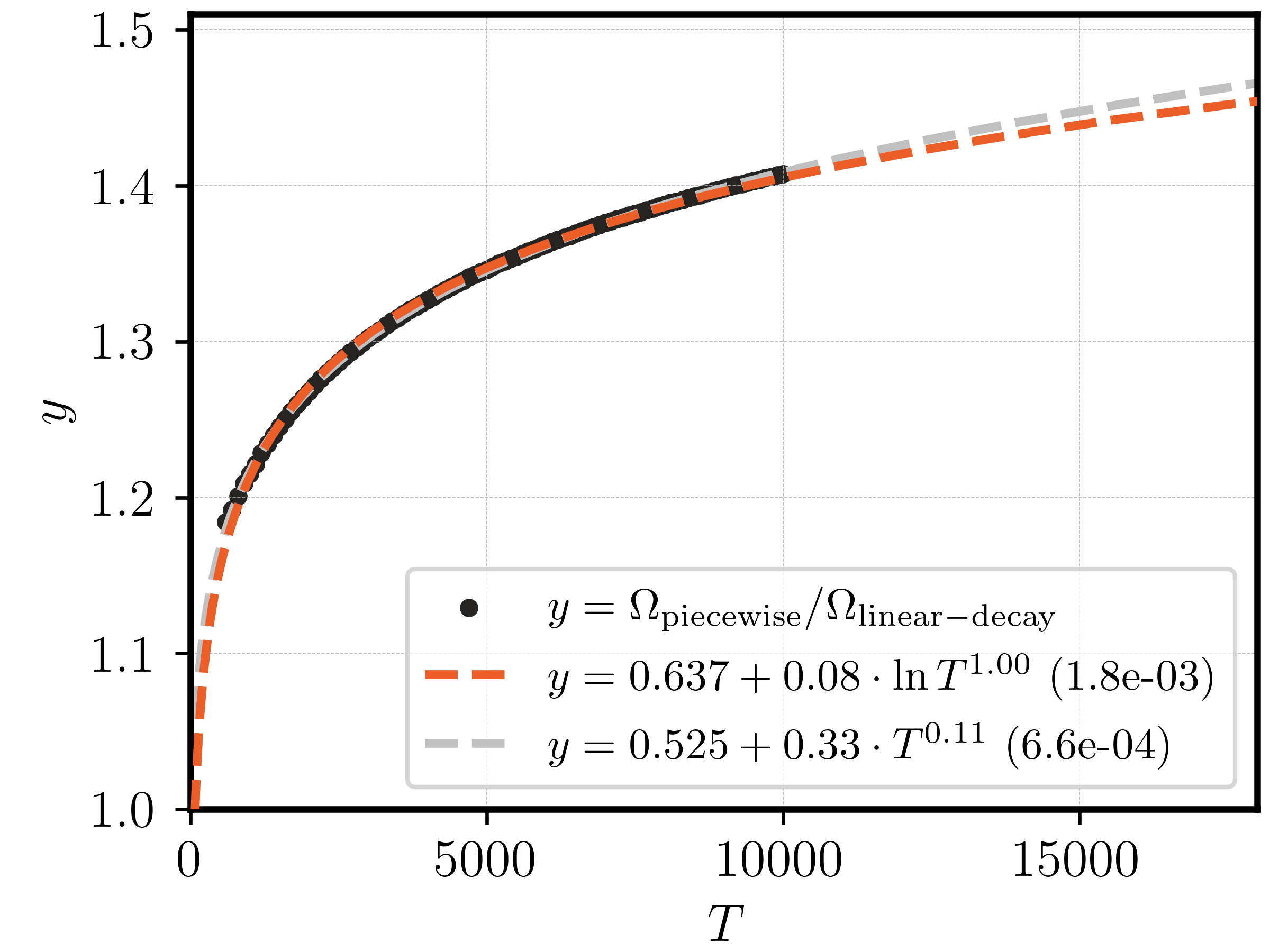
Figure 4: Scaling laws for the performance loss compared to linear-decay. Number in brackets indicates the mean absolute deviation over the data points (black).
Figure 4 shows that both laws fit the data well, with a slight advantage in favor of the standard powerlaw. As it seems intractable to derive the bound in analytical form for the piecewise schedule, we cannot go down any further this road at this point.
Asymptotics of the piecewise constant schedule. Next, we look at the resulting shape of the piecewise constant schedule (again for \(\Delta t=100\)). Figure 5 plots the obtained schedule (left) and its bound (right) compared to the sqrt-schedule. We can see that the schedules look quite similar, and that the piecewise schedule yields a slightly better bound.
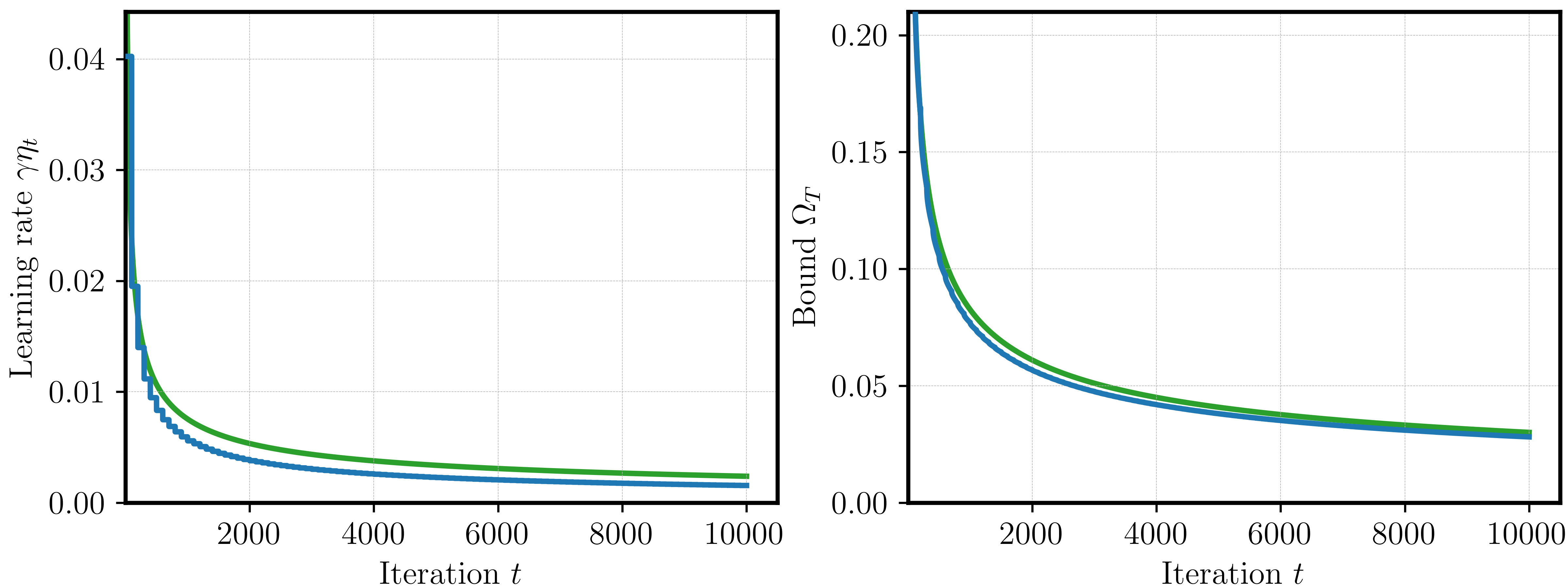
Figure 5: Learning rate (left) and bound (right) for piecewise constant schedule (blue) and sqrt schedule (green).
Again, this suggests that bigger look-ahead (here for piecewise schedule) achieves better bounds. We take a closer look: what happens when the look-ahead advantage vanishes? For this we look at three different values \(\Delta t \in \{20, 100, 500\}\). First, we can see (Figure 6, left) that the sequentially constructed piecewise constant schedule indeed quickly arrives at \(1/\sqrt{t}\).
Second, the advantage of piecewise constant vs. sqrt after a sufficiently large burn-in time also becomes smaller when \(\Delta t\) is smaller (Figure 6, right). However, even with only 20 look-ahead steps we can still obtain a 5% smaller bound.
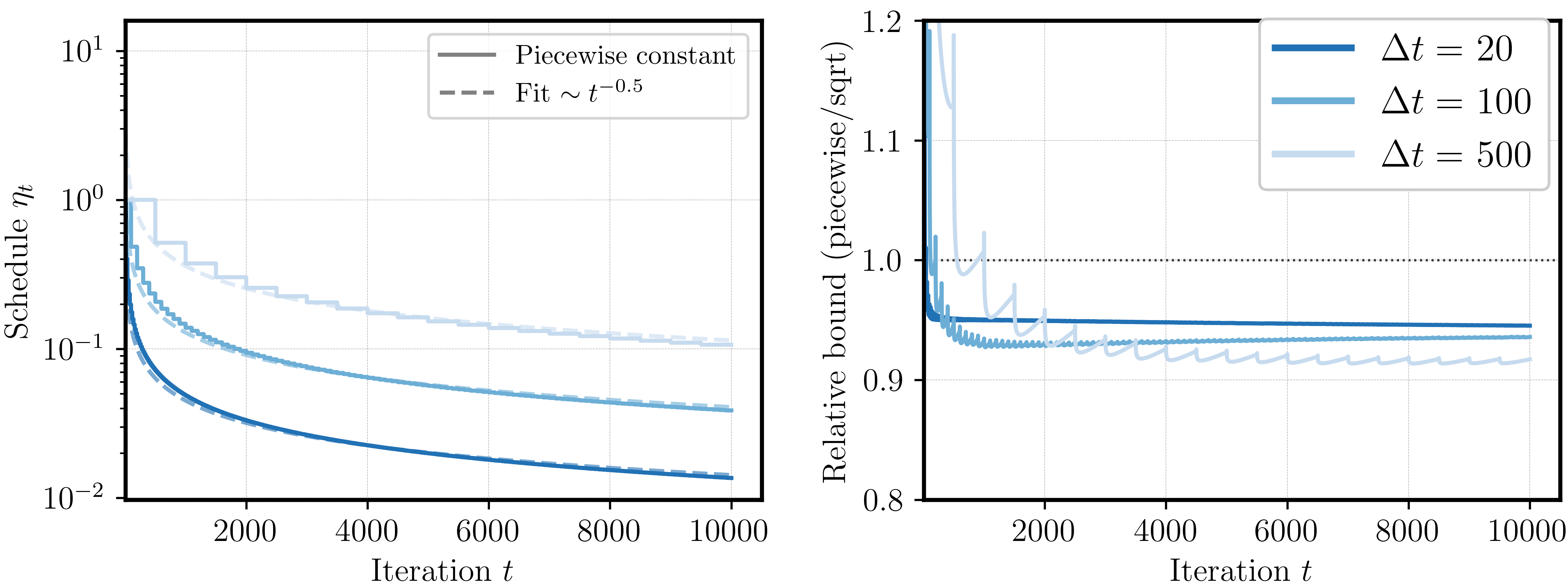
Figure 6: Left: Piecewise constant schedule asymptotic shape. Right: relative improvement for different look-ahead steps.
This leaves us with the following insight: being able to plan ahead for \(\Delta t\) iterations allows to design schedules with better bounds. The sqrt-schedule, which is a textbook example in convex, nonsmooth optimization, comes out naturally as the limiting schedule when \(\Delta t \to 1\).
This connection led me to re-visit how the sqrt-schedule is usually motivated: classical textbooks (e.g. the ones by Nesterov and Polyak) introduce the sqrt-schedule for the subgradient method as the anytime-proxy for the optimal constant step size \(\propto 1/\sqrt{T}\). This structure originates from balancing two terms in the suboptimality bound, where one relates to the sum of step sizes, and the other to the sum of squared stepsizes. I could not find a geometric motivation for the rule \(1/\sqrt{t}\) (let me know, if you know one); it seems that our construction of a piecewise constant schedule refines the classical derivation (from constant \(1/\sqrt{T}\) to anytime \(1/\sqrt{t}\)).
Conclusions
Knowing the training horizon in advance (“lookahead”) allows to design better learning-rate schedules. We can use convex, nonsmooth optimization bounds to design an piecewise constant schedule, that plans ahead from one checkpoint to the next.
Compared to the ideal linear-decay schedule, the drawback of our piecewise constant strategy grows with training length. Compared to the no-lookahead sqrt-schedule, even rather short lookahead still yields a noticeable (theoretical) advantage.
Maybe the most interesting takeaway: the sqrt-schedule appears as the limit of the piecewise constant strategy, when the lookahead vanishes.
Acknowledgements. I’d like to thank Francis Bach for his feedback on this post.

References
Defazio, A., Cutkosky, A., Mehta, H., and Mishchenko, K. Optimal linear decay learning rate schedules and further refinements. arXiv:2310.07831, 2023. [link]
Orabona, F. Last iterate of SGD converges (even in unbounded domains), 2020. [link]
Schaipp, F., Hägele, A., Taylor, A., Simsekli, U., Bach, F. The Surprising Agreement Between Convex Optimization Theory and Learning-Rate Scheduling for Large Model Training. ICML, 2025. [link]
Shamir, O. and Zhang, T. Stochastic gradient descent for non-smooth optimization: Convergence results and optimal averaging schemes. ICML, 2013. [link]
Zamani, M. and Glineur, F. Exact convergence rate of the last iterate in subgradient methods. arXiv:2307.11134, 2023. [link]
Zhai, X., Kolesnikov, A., Houlsby, N., and Beyer, L. Scaling vision transformers. CVPR, 2022. [link]
Appendix
Last-iterate bound for the sqrt-schedule
Orabona (2020) analyses the schedule \(\eta_t = 1/\sqrt{t}\) in the convex, Lipschitz setting. With a slight modification of their analysis (see Cor. 3 therein), if \(G\) denotes the Lipschitz constant of the objective \(f\), then we get
\[\mathbb{E}[f(x_T) - f_\star] \leq \frac{1}{2\sqrt{T}} \big[\frac{D^2}{\gamma} + \gamma G^2(1+\log(T)) + 3\gamma G^2(1+\log(T-1)) \big].\]Minimizing this bound with respect to \(\gamma\), we obtain \(\gamma^\star = \frac{D}{G\sqrt{1+\log(T)+ 3(1+\log(T-1))}}\). Plugging this back into the bound, we obtain
\[\mathbb{E}[f(x_T) - f_\star] \leq \frac{DG}{2\sqrt{T}}\mathcal{O}(\sqrt{\log(T)}).\]We also point towards Shamir and Zhang (2013), who derive the bound \(\frac{DG(2+\log{T})}{\sqrt{T}} \) if \(\gamma=D/G \), however assuming a bounded domain.